Overfitting and out-of-sample: why the best backtest is the one to distrust

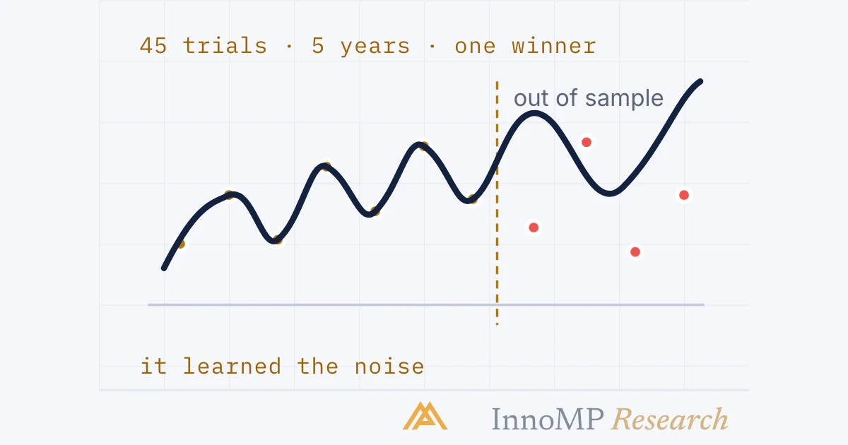
Overfitting is tuning a rule until it fits the noise of the sample it was tested on, so that its record does not carry to new data. It comes from trials, not from any one test — and the number of trials is the part of the evidence that almost never gets written down. The best backtest of many is the one whose numbers mean least.

Parts 11 and 12 assumed one record, honestly kept. This part is about the records that were not kept: the versions of the rule tried and discarded on the way to the one in the notebook. They change what the surviving record means, and the tools for dealing with them are older than trading.

Fitting the signal, fitting the noise

Any set of past trades has two things in it: whatever repeats, and whatever happened once. A rule with enough adjustable parts can be bent to match both.

In a setup the adjustable parts are the parameters: the ATR multiple on the stop, the lookback, the session filter, the minimum pullback depth, the day-of-week exclusion added after a bad Friday. Each is a knob, and each value tried on the same data is a chance to match an accident. Overfitting — curve fitting, in the older phrase — is what the setup has done when its record on the tuning data is excellent and its record on anything else is ordinary or worse. The trader who did it rarely notices, because from inside, every adjustment looked like learning.

The best of N is not the best

The mechanism is not subtle, and a 2014 paper in the Notices of the American Mathematical Society by Bailey, Borwein, López de Prado and Zhu put numbers on it. Suppose a researcher tries N configurations of a strategy, none of which has any real edge — every one has a true Sharpe ratio of zero. The best of the N, measured on the sample, will not show zero. It will show the expected maximum of N chance results, and that number grows with N.

The Sharpe ratio is the finance version of a ratio this group has already used: a mean return divided by the spread of returns, annualised — expectancy over its standard deviation, in the units of Part 11. The paper’s example is ten configurations, all skill-less, whose best is expected to show an in-sample Sharpe ratio of 1.57. A discretionary trader does not compute Sharpe ratios, but the logic transfers without change: the best of ten versions of a setup, tuned on the same year of charts, has an expectancy inflated by the choosing, and the error bars from Part 11 — computed as if it were the only version — are too narrow by an amount that depends on the nine that were thrown away.

That is the whole problem in one sentence. The record of the winner is not evidence about the winner until the count of losers is known.

Minimum backtest length

The paper turns the same arithmetic into a rule of thumb it calls the minimum backtest length: the years of data needed so that the best of N trials is not expected to reach a given in-sample Sharpe ratio by chance alone.

The paper’s own examples are the two in the figure: five years of data support no more than about forty-five independent configurations before a skill-less one is expected to look like a Sharpe ratio of 1; two years support about seven. The authors are careful to say what the number is not. It assumes the trials are independent, which makes it conservative — ten values of the same stop multiple are not ten independent ideas — and it is a necessary condition, not a sufficient one: a backtest can be overfit on a sample far longer than the minimum. What it is, is a first answer to a question most people never ask of a record — how many trials produced it — and the authors’ central complaint is that the number is almost never reported, in academic papers or by anyone selling a result, which makes the risk of overfitting impossible to assess from the result alone.

For a discretionary trader the count is small and the data is short. A year of four-hour charts on two pairs, and a setup whose stop multiple, session filter and pullback depth were each tried at three values, is twenty-seven configurations on one year — already past the paper’s line. The record of the winner may still be fine. It is just not evidence yet.

Hold data out

The oldest remedy is to keep some of the data away from the tuning.

An out-of-sample test is a rule run once, unchanged, on data it was never tuned on. If its out-of-sample record resembles its in-sample one — the same order of expectancy, an interval that overlaps — the rule learned something that persisted past the tuning data. If the record collapses, the in-sample numbers were the noise. The discipline is entirely in the word once: the held-out data is spent the moment it is looked at, and any adjustment made after looking makes the next run in-sample by definition. The paper notes the limit of the method too — a hold-out does not know how many trials came before it, so a rule that survived hold-out is still the best of N in a different sense — but as a first filter it removes most of what the previous section described.

The Intermediate level’s forward test is the same idea with the data supplied by the calendar instead of the archive: demo trades taken in real time cannot have been tuned on, because they had not happened.

Walk forward

A single split spends the data once. Walking forward spends it repeatedly and gets a longer out-of-sample record for the same history.

A walk-forward test is an out-of-sample test repeated through the history: tune on the first window, test on the period after it, slide both forward by the length of the test period, and stitch the test periods together. The stitched record has the property that matters — no part of it was tuned on — and it is long enough to have error bars of its own. It also produces something a single split does not: the sequence of parameters chosen in each window. If the stop multiple that tested best is 1.5 in one window, 2.5 in the next and 1.2 in the third, the rule has no stable parameter, and re-tuning it each window is the overfitting, done on a schedule.

Plateau, not peak

The last defence is about how a parameter is chosen inside a window, and it needs no held-out data at all.

Sweep a parameter across its plausible range and draw the result against it. A rule that works has a plateau: a stretch of values where the result is similar, because the market feature the rule captures is not sensitive to the exact number. A rule fit to noise has a peak: one value that is much better than its neighbours, because that value happened to catch this sample’s accidents. The peak is always the maximum, which is why choosing the maximum is the mistake. Choose a value inside the plateau — the middle of it, not the best point on it — and the rule loses a little on the tuning data and keeps most of it elsewhere.

The trial log

Everything above reduces to one addition to the journal the Intermediate level built: a log of trials. Every configuration tried, the data it was tried on, its result, and why it was dropped — including the ones that were only tried in the head for an afternoon and abandoned, since the paper’s point is that those count. The log does three things. It gives N, so that the survivor’s numbers can be read against the number of losers. It records the parameter sweeps, so that a peak can be told from a plateau later, when the sample is longer. And it makes the adjustments visible as adjustments, which is the only defence against the feeling, from inside, that each one was learning.

The paper’s last observation is the one to end on. When trials are not counted, a good backtest is not merely uninformative; on data with memory — where a period that was fit to tends to be followed by its opposite — the authors show the out-of-sample expectation of an overfit rule is negative. The customary warning that past performance does not indicate future results, they write, is too optimistic in that setting. A record that was chosen is not a weak signal. It can be a signal pointing the wrong way.

Where this leaves the record

The group is finished. A record now carries three things it did not carry at the end of the Intermediate level: error bars on its expectancy, a distribution around its drawdown, and a count of the trials behind it. A setup whose interval clears costs, whose drawdown tail is sized for, and whose trial count is small and written down has an edge in the only sense this level uses the word. The last group of the level — Parts 14 to 16 — takes a setup that has passed and turns it into something that can be run: a decision table, alert and execution rules, and a review cadence with the criteria for switching it off.

Next: From rules to a decision table — every state of the market gets a column, and the gaps and contradictions the prose hid come out.

Trading journal Discipline Risk management