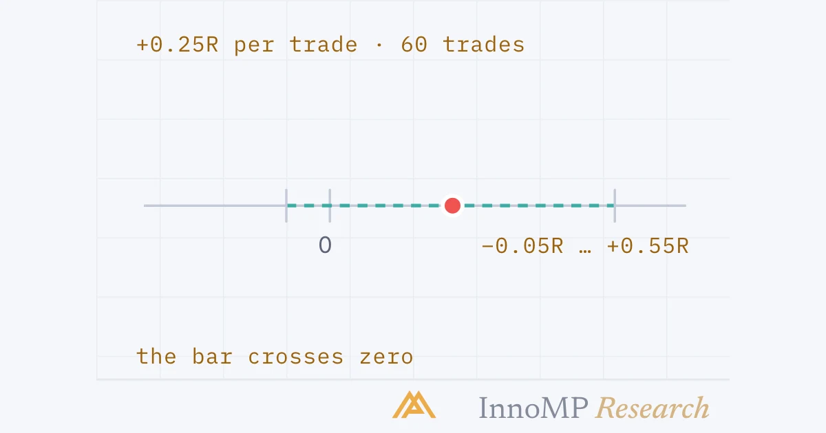
Expectancy with error bars means reporting the mean R per trade together with its standard error — the spread of the trade results divided by the square root of the number of trades — and the confidence interval that follows from it. A record of 60 trades averaging +0.25R with a 1.2R spread has a standard error near 0.15R, so the 95% interval runs from about −0.05R to +0.55R: the edge cannot yet be told from none. The interval narrows with the square root of the sample, so halving it takes four times the trades.
Expectancy with error bars means reporting the mean R per trade together with its standard error, and the confidence interval that follows from it — so that a record is read as a range rather than a number. A record of sixty trades at +0.25R has not shown an edge. It has shown a number whose error bar reaches below zero.
The Intermediate level ended with a notebook: every trade a setup would have taken, and the arithmetic that turns the list into a win rate, an average win and loss, and an expectancy. That part gave the win rate its error bars. This group does the same for the number that matters — the expectancy itself — and then asks the two questions a record cannot answer on its own: how bad its drawdowns could have been, and whether the rules were fitted to the past they were tested on.
The record is a sample
Sixty trades is a sample of a process. Run the same setup on a different sixty — the next year, a different pair — and the mean comes out somewhere else. The distance it typically moves is the standard error: the standard deviation of the individual trade results, in R, divided by the square root of the number of trades.
The confidence interval is the mean plus or minus a multiple of the standard error — for a 95% interval, a t-value that is close to two once the sample is beyond a few dozen trades. The NIST handbook is precise about what it means, and the precision matters: it is not a 95% probability that the true expectancy is inside this bar. It is that if many records of sixty were collected and the interval computed for each, about 95% of those intervals would contain the true value. This one is one of them, and whether it is among the 95% or the 5% cannot be known from inside it.
What can be known is its width, and the width is the point. An interval from −0.05R to +0.55R contains a setup that loses slowly, a setup that makes half an R a trade, and everything between. The record has narrowed the possibilities; it has not chosen among them.
Why the square root
The standard error shrinks with the square root of the sample, not with the sample. Doubling the record does not halve the bar.
This is the arithmetic under a rule the Intermediate level stated without it: more trades than feels necessary. It is also why the win-rate interval that part quoted — about eighteen points either way at thirty trades, about six at three hundred — has the shape it has. The win rate is a proportion, and a proportion’s standard error shrinks by the same square root.
The spread matters as much as the count
The other term in the standard error is the spread of the results, and the spread is a property of the setup — of how it exits — not of the market.
A setup that loses 1R and wins 1.5R has results that sit close to their mean. A setup that loses 1R and occasionally wins 6R — the trend-following shape, where most trades scratch and a few pay for the year — has a spread more than twice as wide, and its standard error is more than twice as large at any sample. The second setup can have the higher expectancy and still be the harder one to prove. This is not a reason to prefer either; it is a reason to know which one is in the notebook before deciding how much the notebook can say.
Reading the interval
Once the interval is drawn there are only three things it can be doing relative to zero.
This is the sense in which the level uses the word. An edge is a positive expectancy that stays positive after spread and swap and whose confidence interval sits above zero. A positive number on its own is not one; it is record B, and record B is what almost every record looks like at the size a hand replay produces. The honest reading of B is not “it works” or “it doesn’t” but “keep counting” — which is a decision about time and demo trades, not about money.
Costs move it; the sample narrows it
The interval was drawn on gross results. The real cost of a trade — spread, swap, slippage — comes off every one of them, and in R it is a fixed amount per trade for a given setup, because the stop is a fixed multiple of the same things.
Two consequences. A setup with a small gross edge can have none at all net, and the record will not reveal it until costs are entered trade by trade — which is why the Intermediate level’s notebook has a column for them. And the comparison between two setups is a comparison of net intervals: a setup that trades more often pays the cost more often, and its interval is lower by more.
Key takeaway A record’s expectancy is a point; its standard error is the spread of results over the square root of the count; the confidence interval is roughly two of those either side. Costs move the interval down. Only more trades — many more — make it narrower. The setup has an edge when the bar sits above zero after costs, and not before.
How many trades
The question the Intermediate level answered with “more than feels necessary” has an arithmetic answer, and it is worth seeing because it is larger than intuition allows.
The left column is the standard error turned around: the sample at which two standard errors equal the expectancy, so that the interval would just exclude zero if the record’s mean were the truth. The right column is the NIST handbook’s formula for the sample needed to detect a shift of a given size — the sum of two z-values, squared, times the spread over the shift, squared — with the conventional 5% chance of a false positive and 10% chance of a miss. It is about two and a half times the left column, because it asks not merely that the bar could clear zero but that it will, nine times in ten.
Either column says the same thing about small edges. An expectancy of a tenth of an R is a real edge — over a thousand trades it is a hundred R — and it is also one that a setup firing twice a week cannot demonstrate inside five years. The setups that can be validated by a discretionary record are the ones whose edge per trade is large relative to the spread of their results. That is a constraint on what this level can honestly call an edge, and it is better known before the notebook is opened than after.
What the interval cannot say
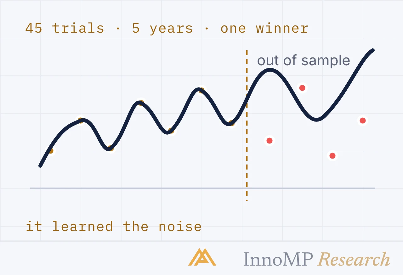
The interval describes the mean, and it treats the record as a bag of independent results whose order does not matter. Two things escape it. The order of the trades does matter, to everything about drawdown — a record with a fine expectancy can still have arrived by a path the trader could not have sat through, and the next part resamples the record to see how bad the other paths were. And the record is assumed to be the only one: if it is the best of ten versions of the rule, the interval is too narrow by an amount that depends on the ten, which is where the group ends.
Next: Monte Carlo and drawdown — resampling the record’s trades to see the drawdowns its order hid, and sizing so that the bad draws are survivable.
- Expectancy is the mean R per trade; its standard error is the standard deviation of the trade results divided by the square root of the number of trades.
- A confidence interval for a mean is the mean plus or minus a t-value times the standard error, and it narrows with the square root of the sample (NIST e-Handbook).
- Illustrative: 60 trades at +0.25R with a 1.2R spread give a 95% interval of about −0.05R to +0.55R; 300 trades narrow it to about +0.11R to +0.39R.
- Four times the trades halve the error bar; the same precision on a smaller edge needs proportionally more trades.
- Spread and swap shift the whole interval down without narrowing it, so an edge is judged after costs.