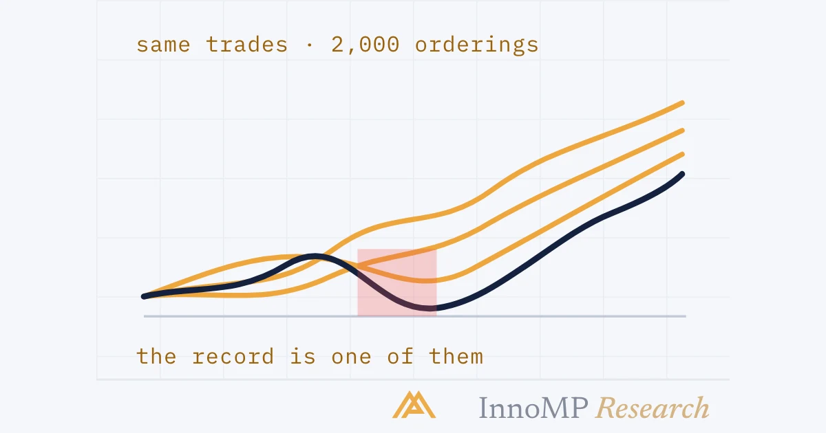
A Monte Carlo test resamples the trades in a record thousands of times, with replacement, and records the maximum drawdown and longest losing run of each resampled path. The record's own drawdown is one path among them, usually near the middle of the distribution, not its tail. Illustrative: a 300-trade record at 1% risk whose own drawdown was 6.8% gave, over 2,000 resamples, a median near 7%, a 95th percentile near 11% and a tail above 18%. Size so that the tail is survivable, not the record.
A Monte Carlo test resamples the trades in a record thousands of times and measures each resampled sequence for the things that depend on order — maximum drawdown, longest losing run — so that the record’s own worst stretch is read as one draw among many rather than as the worst case. The record’s drawdown is usually near the middle of that distribution. The number to plan around is in its tail.
Part 11 put error bars on the mean, and the mean does not care what order the trades came in. Drawdown does. The Intermediate level said that the longest losing run in a record is a lower bound on what the setup will produce; this part is why, and by how much.
One record is one ordering
Take a record of three hundred trades: 45% winners at +2R, the rest −1R, risked at 1% of equity each. Its equity curve rises, and somewhere along it there is a worst stretch.
The maximum drawdown is the largest peak-to-trough fall the curve shows, as a percentage of the peak — the same measurement the psychology series applied to a live account, applied here to a record. Here it is 6.8%. That number went into the notebook, and a trader who plans to survive a 6.8% drawdown has planned for this ordering and no other.
The same three hundred results in a different order give a different curve. Nothing about the setup has changed — the win rate, the R-multiples, the expectancy and its error bars are identical, because none of them depends on order — and yet the curve can be shallow or brutal depending on where the losses landed. The trader lives through one ordering, and which one is not in the setup’s gift.
Resampling the record
The tool for seeing the other orderings is the bootstrap. The NIST handbook describes it plainly: draw subsamples from the data with replacement, so any observation can appear several times or not at all; compute the statistic for each; repeat, typically five hundred to a thousand times; and the computed values form an estimate of the statistic’s sampling distribution.
Bootstrap resampling applied to a trade record is exactly this: the results are the data, a resampled path is three hundred draws from them with replacement, and the statistics computed for each path are the ones that depend on order — maximum drawdown, longest losing run, time from one equity high to the next. A Monte Carlo simulation is the general name for the practice of generating many such paths and reading their distribution; shuffling the record without replacement is the other common form, and keeps the exact set of results while changing only their order. For a record of this size the two give similar answers, and the bootstrap has the advantage that it also lets the mix of wins and losses vary a little, as it would in a new sample.
None of this needs a statistics package. A spreadsheet that holds the results in one column and a random draw from them in the next, recalculated a thousand times with the worst dip noted each time, is the whole method.
The distribution
Run it and the record’s drawdown becomes a point on a histogram.
The numbers are illustrative — one record, one run — but the shape is what every record produces. The record’s own drawdown lands near the middle, because the record is an ordinary draw from its own distribution, and ordinary draws land in the middle. The tail is where the planning number is: the 95th percentile says that one path in twenty was worse than about 11%, and a trader who plans to survive the record’s 6.8% has planned for a path better than most.
Which percentile to plan around is a decision, not a statistic. The 95th is common; the worst path is not, because the worst of two thousand is itself a lucky draw, of the other kind.
Losing runs
The same resampling answers the question the psychology series raised with coin flips: how long a losing run to expect. With a 55% chance of a loss on any trade, the probability of eight in a row starting from a given trade is 0.55 to the eighth power — about one in 120. That sounds rare until it meets the number of chances.
So a setup with a 45% win rate — a perfectly good one at 2R — should be expected to lose eight times in a row somewhere in its first three hundred trades, and twelve in a row is not a surprise but a bad year. The Intermediate level said the record’s longest run was a lower bound; the resample says how much room is above it. It also says something the record cannot: that the run is a property of the win rate and the sample length, and not of anything the trader did wrong in the week it happened.
Size decides what a run costs
The run is the setup’s. What it costs is the sizing’s — which is the previous part’s point from the other side. Twelve consecutive losses at a fixed fraction of equity compound:
This is how the distribution becomes a sizing rule. Choose the percentile to survive — say the 95th — and read its drawdown at the risk per trade the simulation assumed. If it is deeper than the plan tolerates, lower the risk and rerun; at fixed-fraction sizing the drawdown from a given run moves roughly in proportion to the risk, so halving the risk roughly halves the tail. The position size calculator turns the chosen risk back into lots once the stop is known.
Read the other way, the same arithmetic explains why the psychology series spends three parts on drawdown. A 30% hole is not survived by discipline; it is avoided by having sized for the twelve-loss run before it arrived, when it was still a bar on a histogram.
Key takeaway The record’s drawdown is one ordering of its results. Resample the results a few thousand times, take the maximum drawdown and longest losing run of each path, and plan around a percentile of that distribution, not the record. Then size so that the drawdown at that percentile is one the plan can hold.
What resampling assumes
Every resampled path treats each trade as independent of the last — a fresh draw from the same bag. Real records are not like that, and the previous group said why: volatility clusters, and a setup that fails in a regime tends to keep failing while the regime lasts.
So the resampled distribution is optimistic in a specific direction: real runs are longer and real drawdowns deeper than independent draws produce, because the losses arrive together. The honest use of the histogram is as a floor — the least bad the bad paths get — and the honest response to the floor is to size for a tail beyond it, or to add the regime as a condition of the setup so that the clustered losses are not taken at all, which is a change to the rules that the next part has something to say about.
The next part is about the other way a record lies: not by its order, but by having been chosen.
Next: Overfitting and out-of-sample — why the best of many backtests is the one to distrust, and how held-out data and walking forward tell fit from luck.
- Bootstrap resampling draws subsamples with replacement from the data and computes the statistic for each, typically 500 to 1,000 times (NIST e-Handbook).
- Applied to a trade record, each resample is a new ordering of the same results; its maximum drawdown and longest losing run are what get recorded.
- The record's own maximum drawdown is one draw from that distribution, usually near its middle rather than its tail.
- With a 55% loss rate, eight losses in a row has a probability near 1 in 120 from any given trade, so a 300-trade record is expected to contain such a run.
- Twelve consecutive 1% losses compound to an 11.4% drawdown; at 2% risk the same run is 21.5%, at 3% it is 30.6%.
- Resampling assumes trades are independent; volatility clustering makes real runs longer than the resample says, so its answer is a floor.